Winter Crops Optimization with Area Bounds
WinterCropsAreaBounds.RmdProblem Statement
A Mediterranean farm has 15 ha of land, 350 h of labor and 500 kg of available nitrogen. It can grow four winter crops:
Oat (a gramineae)
Barley (a gramineae)
Fava bean (a legume)
Lupin (a legume)
Crop data (per ha):
| Crop | N fertilizer (kg) | Labor (h) | Gross margin (€) |
|---|---|---|---|
| Oat | 80 | 20 | 400 |
| Barley | 100 | 25 | 450 |
| Lupin | 0 | 15 | 350 |
| Fava bean | 30 | 30 | 500 |
We wish to maximize total gross margin subject to resource constraints. Furthermore, each crop has a required area range (ha):
Oat: 2 ≤ area ≤ 8
Barley: 1 ≤ area ≤ 6
Fava: 3 ≤ area ≤ 7
Lupin: 2 ≤ area ≤ 5
Step 1: Define Resource Constraints (flexible min/max for each crop)
# Step 1: Define Resource Constraints (flexible min/max for each crop)
resources <- define_resources(
  resources = c(
    # global totals
    "land", "labor", "nitrogen",
    # per‐crop bounds
    "oat_min",   "oat_max",
    "barley_min","barley_max",
    "lupin_min", "lupin_max",
    "fava_min",  "fava_max"
  ),
  availability = c(
    # totals
     15,    350,    500,
    #  bounds
      2,      8,
      1,      6,
      3,      7,
      2,      5
  ),
  direction = c(
    # totals all <=
    "<=",   "<=",   "<=",
    # minimums >=
    ">=",   "<=",
    ">=",   "<=",
    ">=",   "<=",
    ">=",   "<="
  )
)

print(resources)
#>      resource availability direction
#> 1        land           15        <=
#> 2       labor          350        <=
#> 3    nitrogen          500        <=
#> 4     oat_min            2        >=
#> 5     oat_max            8        <=
#> 6  barley_min            1        >=
#> 7  barley_max            6        <=
#> 8   lupin_min            3        >=
#> 9   lupin_max            7        <=
#> 10   fava_min            2        >=
#> 11   fava_max            5        <=
Step 2: Define Activities (Crop Choices)
# Step 2: Define Activities
activity_requirements_matrix <- matrix(
  c(
    # land usage (ha/ha)
     1, 1, 1, 1,
    # labor   (h/ha)
    20,25,15,30,
    # nitrogen (kg N/ha)
    80,100, 0,30,
    # bounds rows for technical matrix:
    #   for oat_min  (1 for oat else 0)
     1,0,0,0,
    #   for oat_max
     1,0,0,0,
    # barley_min
     0,1,0,0,
    # barley_max
     0,1,0,0,
    # fava_min
     0,0,1,0,
    # fava_max
     0,0,1,0,
    # lupin_min
     0,0,0,1,
    # lupin_max
     0,0,0,1
  ),
  nrow = nrow(resources),
  byrow = TRUE,
  dimnames = list(
    resources$resource,
    c("oat", "barley", "lupin", "fava")
  )
)

objective <- c(oat = 400, barley = 450, lupin = 350, fava = 500)

activities <- define_activities(
  activities = colnames(activity_requirements_matrix),
  activity_requirements_matrix = activity_requirements_matrix,
  objective = objective
)

activities
#>        activity land labor nitrogen oat_min oat_max barley_min barley_max
#> oat         oat    1    20       80       1       1          0          0
#> barley   barley    1    25      100       0       0          1          1
#> lupin     lupin    1    15        0       0       0          0          0
#> fava       fava    1    30       30       0       0          0          0
#>        lupin_min lupin_max fava_min fava_max objective
#> oat            0         0        0        0       400
#> barley         0         0        0        0       450
#> lupin          1         1        0        0       350
#> fava           0         0        1        1       500
Step 3: Build and Solve the Model
# Step 3: Build and Solve the Model
model <- create_ram_model(resources, activities)
solution <- solve_ram(model, direction = "max")
Step 4: Results
dat <- data.frame(
  activity = names(solution$optimal_activities),
  level    = round(as.numeric(solution$optimal_activities), 1)
)

DT::datatable(
  dat,
  rownames = FALSE,
  options = list(
    autoWidth = TRUE,
    columnDefs = list(
      list(width = '2cm', targets = 0),  # first column (activity)
      list(width = '2cm', targets = 1)   # second column (level)
    )
  )
) |>
  DT::formatRound(
    columns = "level",
    digits  = 2
  )
Step 4: Results
summary_ram(solution)
cat("Maximum gross margin (EUR):", solution$objective_value, "\n")
#> Maximum gross margin (EUR): 6290
plot_ram(solution)Scenario Analysis
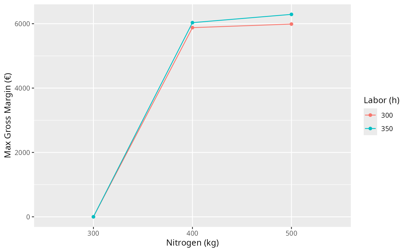
Below we explore what happens if we vary total nitrogen and labour availability.
library(ram)

# 1) Re‐load your data.frames from the vignette/example:
resources   # data.frame with columns resource, availability, direction
#>      resource availability direction
#> 1        land           15        <=
#> 2       labor          350        <=
#> 3    nitrogen          500        <=
#> 4     oat_min            2        >=
#> 5     oat_max            8        <=
#> 6  barley_min            1        >=
#> 7  barley_max            6        <=
#> 8   lupin_min            3        >=
#> 9   lupin_max            7        <=
#> 10   fava_min            2        >=
#> 11   fava_max            5        <=
activities  # data.frame with columns activity, land, labor, nitrogen, …, objective
#>        activity land labor nitrogen oat_min oat_max barley_min barley_max
#> oat         oat    1    20       80       1       1          0          0
#> barley   barley    1    25      100       0       0          1          1
#> lupin     lupin    1    15        0       0       0          0          0
#> fava       fava    1    30       30       0       0          0          0
#>        lupin_min lupin_max fava_min fava_max objective
#> oat            0         0        0        0       400
#> barley         0         0        0        0       450
#> lupin          1         1        0        0       350
#> fava           0         0        1        1       500

# 2) Build the ram specs:
res0 <- define_resources(
  resources    = resources$resource,
  availability = resources$availability,
  direction    = resources$direction
)

# NOTE THE TRANSPOSE HERE!
tech_mat <- t( as.matrix(
   activities[, setdiff(names(activities), c("activity","objective"))]
) )

act0 <- define_activities(
  activities                   = activities$activity,
  activity_requirements_matrix = tech_mat,
  objective                    = activities$objective
)

# 3) Define your scenario grid:
scenarios <- list(
  nitrogen = c(300, 400, 500),
  labor    = c(300, 350)
)

# 4) Run them:
scen_df <- run_scenarios(res0, act0, scenarios, direction = "max")
print(scen_df)
#>   nitrogen labor objective      oat barley lupin     fava
#> 1      300   300     0.000 0.000000    0.0   0.0 0.000000
#> 2      400   300  5877.778 2.166667    1.0   7.0 4.222222
#> 3      500   300  5988.889 3.833333    1.0   7.0 3.111111
#> 4      300   350     0.000 0.000000    0.0   0.0 0.000000
#> 5      400   350  6033.333 2.000000    1.0   7.0 4.666667
#> 6      500   350  6290.000 2.000000    1.9   6.1 5.000000
library(ggplot2)
ggplot(scen_df, aes(x=factor(nitrogen), y=objective, color=factor(labor), group=factor(labor))) +
  geom_line() + geom_point() +
  labs(x="Nitrogen (kg)", y="Max Gross Margin (€)", color="Labor (h)")